- awesome MLSS Newsletter
- Posts
- The Transformer Highway now has more off-ramps - Awesome MLSS Newsletter
The Transformer Highway now has more off-ramps - Awesome MLSS Newsletter
17th Edition
Awesome MLSS
March 29, 2026

As we enter our 17th Edition, you may have noticed we often link back to our older articles when explaining new concepts. Transformers do this too - they use residuals to pass information from previous layers.
For the most part, residuals remain a relatively underexplored field - we have worked hard on attention, on FFNs, and other components of the transformer, but rarely the residuals.
A new paper by Moonshot AI, the creators of the Kimi model series explores a new way of calculating residuals. More on this after some updates.
Upcoming Summer School Announcements
Applications for some of the following summer schools are closing in the next 10 days. Make sure to apply to them before the application deadline!
Title | Deadline | Dates |
Mar 31 | Aug 3 - Aug 7 | |
Apr 07 | May 7 - May 16 | |
School on Analytical Connectionism 2026 - Gothenberg, Sweden | Apr 17 | Aug 17 - Aug 28 |
Machine Learning Summer School on Reliability & Safety 2026 - Krakow, Poland | Apr 19 | Jun 29 - Jul 3 |
For the complete list, please visit our website
What’s happening in AI?
Remember, the residual stream is the ‘Add’ part of the add and norm operation in transformers. Below is an example of pre-norm architecture (where we normalize the incoming input before passing it through the layer). The original transformers architecture had post norm, which normalized outputs after passing it through the layer.
The below is a general intuition, Kimi architecture uses a different attention mechanism. However, the same principles apply.
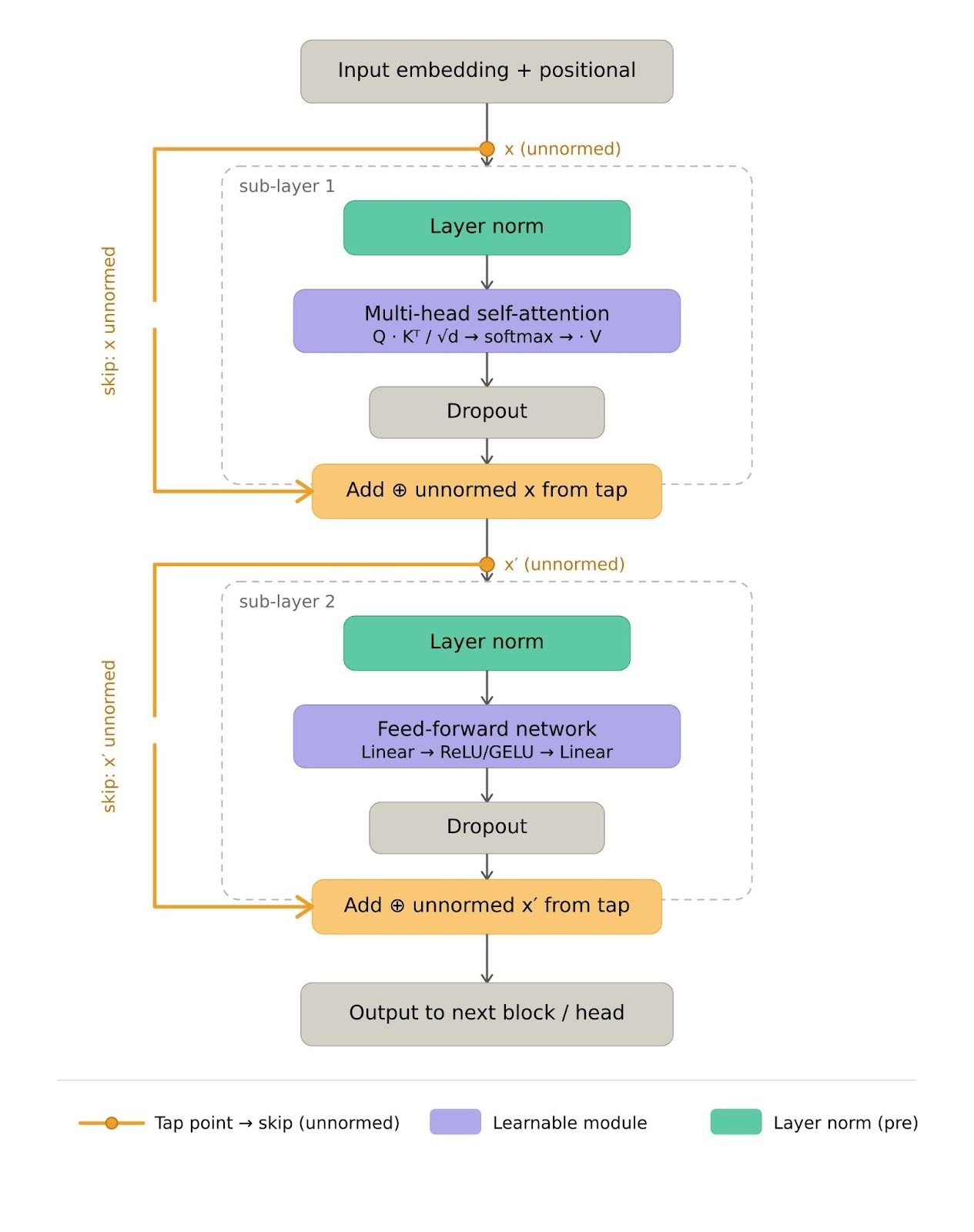
PreNorm SDPA Example. Orange lines and blocks show residual connection. Img Credits: Generated with Claude
Why do we even need residuals? Well, it is mainly to enable gradients to flow along a separate path to allow information capture from the last layer, and avoid the vanishing/exploding gradient problem. As we go deeper in the network, the future layers start losing correlation with past ones - residuals provide a separate pathway independent of the layers. We recommend reading section 2.1 of the paper for a more mathematical treatment.
However, this poses some issues:
There is no selective access - different layer types (FFN, attention) receive the same aggregated state, even if they could potentially benefit from different information recovery
Information lost through aggregation cannot be selectively recovered in future layers
Later layers tend to have extremely large output magnitudes to gain influence of the accumulated residual, destabilizing training
Therefore, the authors propose a new mechanism which allows for self determined selection of what information is needed from which layer.
Unless otherwise mentioned, all image credits go to the original paper, available at https://arxiv.org/pdf/2603.15031
Attention Residuals
In order to provide selective access to the previous layer’s outputs, the authors propose a higher order attention mechanism which determines which layer must be attended to and how much. In effect, as an example for layer 20, it can choose whether or not it attends to layer 4, since different layers have different granularity of analysis using an additional attention layer that attends across layers instead of tokens.
Mind you, this is not an entirely new idea. Cross-layer connectivity and residual stream connections were explored in DenseNet, ELMo, Highway Networks, and many other papers. What is new here is the precise mechanism through which this is achieved. In particular, the authors state that this presents a more unified view of both layer depth, and time in the sequence. Unlike sequence length which can reach millions of tokens, layer depth is typically constrained at much smaller values (L < 1000) making the O(L2) attention over depth feasible computationally.

Formulation
Attention weights over previous layers are defined as

Where the kernel function is defined as φ(q, k) = exp(qᵀ RMSNorm(k)). The RMSNorm in particular prevents layers with large magnitude outputs from dominating the attention weights. The authors note that different designs of the kernel function will behave differently.
For each layer, queries and keys are calculated as

Therefore, the query is a simple learned matrix, independent of incoming inputs. This is an important architectural choice since it allows attention weights for any group of layers to be computed in parallel without waiting for their sequential outputs. Keys and values are kept equal and input dependent. As is evident from the formula, the first layer will directly receive the input embeddings from the embedding layer, while the remaining layers will receive a function dependent output of the last layers - to be discussed soon.
The input to layer l then becomes:

This is the formulation for Full AttnRes, where each layer’s outputs are taken into consideration directly. Per token, we require O(L2d) compute and O(Ld) memory to store layer outputs where d is the hidden dimension of the tokens. As mentioned, L is typically much smaller than sequence length, so the cost is modest, but the authors further optimize this with Blockwise AttnRes, in which we consider blocks of layers.
Each block internally computes AttnRes similar to Full AttnRes, but when it comes to inter-block communication, only the final output state is shared with the downstream blocks. This reduces memory from O(Ld) to O(Nd) and compute from O(L2d) to O(N2d) where N is the number of blocks. There is also reduced inter-node communication from the resultant minimization.
Infrastructure Design
Making the training feasible requires a lot of practical engineering. Imagine a datacenter for training, with several nodes. Each node hosts several GPUs connected to each other through extremely fast transfer speeds, while inter node bandwidth is relatively slower.
For small scale training, the overhead that comes from AttnRes is small and adds no extra memory usage since the activations need to be stored for backprop in any case. However, for large scale training, this overhead is significant - the main challenges arise from pipeline parallelism.
In pipeline parallelism, we have layers distributed sequentially across multiple nodes. For each batch, we first process the first node’s layers, then pass the resultant outputs to the next node, which takes care of processing the next set of layers. The transfer for L layer outputs causes significant transfer, compute and memory overheads. Even with Block AttnRes, this needs to be optimized.
Interleaved Pipelining
Imagine 4 GPUs with 8 layers total. In standard pipeline parallelism each GPU owns a contiguous block:
GPU 1 | GPU 2 | GPU 3 | GPU 4 |
L1, L2 | L3, L4 | L5, L6 | L7, L8 |
The problem is that GPU 1 finishes its forward pass and then sits idle while the activation propagates through GPUs 2, 3, and 4. This idle time is called the pipeline bubble, and it grows with the number of pipeline stages.
With interleaved pipelining, such as implemented in NVIDIA’s NeMo Framework, each GPU is assigned multiple non-contiguous virtual stages instead of one contiguous block:
GPU 1 | GPU 2 | GPU 3 | GPU 4 |
L1, L5 | L2, L6 | L3, L7 | L4, L8 |
This keeps all GPUs busier without violating layer dependencies: a GPU never processes a later virtual stage for a microbatch until the earlier stages have completed for that same microbatch. The result is a smaller pipeline bubble and higher GPU utilization overall.
A further optimization this enables is cross-stage caching: since a GPU holds multiple virtual stages, activations computed in an earlier stage can be reused when that same GPU later processes its later virtual stage, reducing redundant recomputation and communication. This communication cost can be very high for extremely large models.
Inference Optimization
The computation here is performed in two phases. Remember that Full AttnRes is just the extreme case of Blockwise AttnRes where each layer is its own block, so the same theory applies to both. Assume that the size of each block is S. The block representations serve as a shared KV cache that is reused across all layers. The queries are learned weights, and need not be recomputed - they are stored and used as a matrix.
Phase 1: Compute inter-block attention for all S layers simultaneously via a single batched query against the cached block representations, returning both outputs and softmax statistics. This is done to reduce reads from S times to just once per block
Phase 2: Compute the intra-block attention sequentially for each layer using the evolving sum, and then merge these with the phase 1 outputs using the cached softmax statistics and outputs.
Memory Efficient Prefilling
Note that token representations are independent of each other. If we have sequence length T, and hidden dim d, for N block representations, we have Ntd elements, incurring 15GB of memory for a 128k long sequence with 8 blocks. Since the tokens are independent, instead, we shard them by sequence dimension along tensor parallel devices (i.e. all devices are on the same node, high speed bandwidth). We compute the softmax statistics for each chunk of the sequence, then merge these results at the end. This way, the per-GPU memory can be lowered from 15GB to roughly 1.9GB per device (assuming 8 H100 GPUs per node). With chunked prefill, at 16k chunk size, the overhead can be further reduced to 0.3GB per device.
Experiments
The authors use the Kimi Linear architecture, details of which can be found here. There is only one RMSNorm and one pseudo-query vector per layer, initialised to 0 to allow uniformity across all layers
Scaling Laws
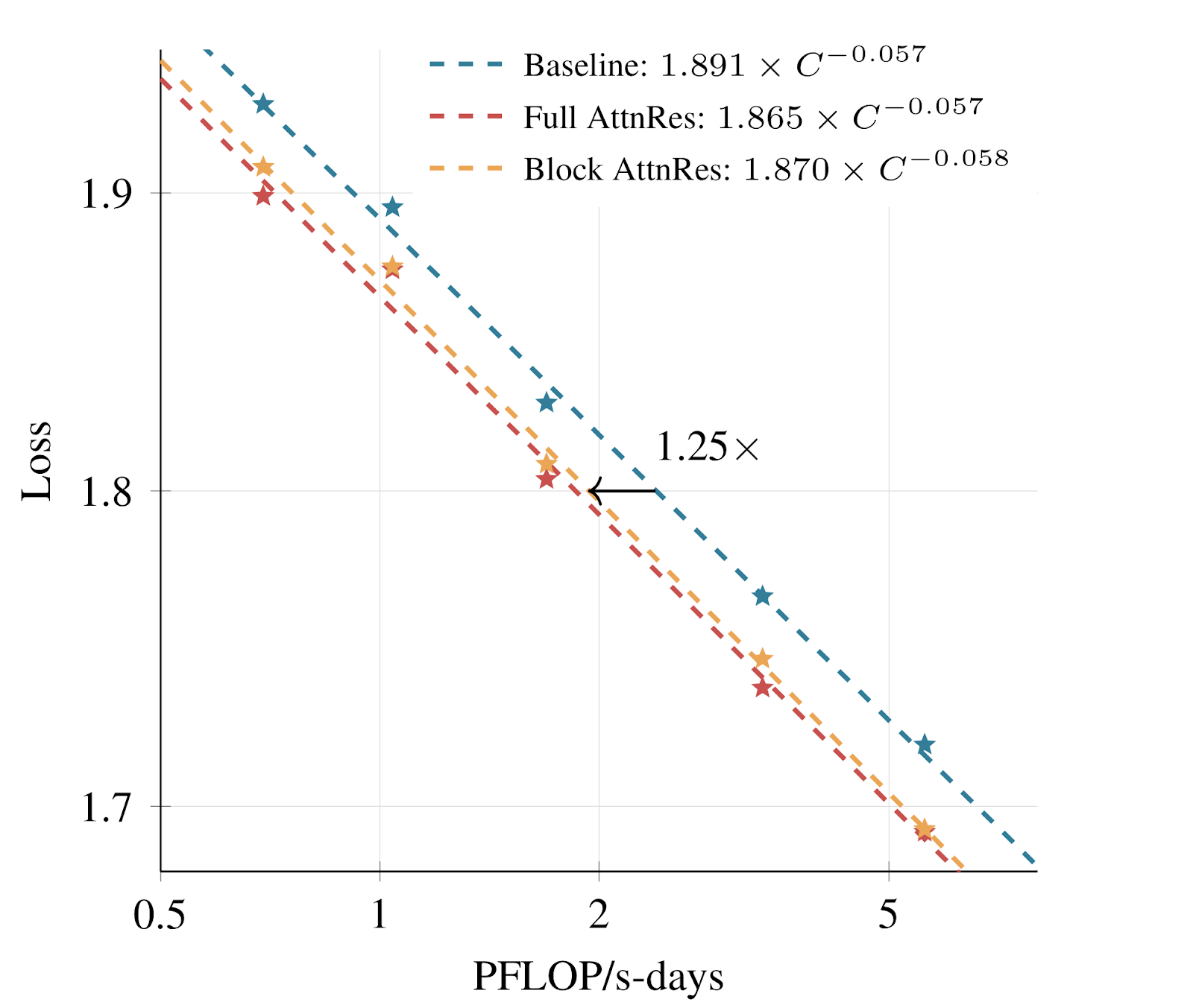
Sweeping across five model sizes for three variants per size - PreNorm baseline, Full AttnRes and Block AttnRes (8 blocks) - the authors fit power law curves L = A x C- alpha where L is validation loss and C is compute measure in PFLOPs-days. By comparing where each curve sits given a fixed compute budget, we can find how much additional compute would be needed for the baseline to match AttnRes loss. Based on experiments, Full AttnRes shows a 1.25x compute advantage over PreNorm baseline, indicating that baseline needs 25% more compute to achieve the same loss as Full AttnRes.
The below is a log-log plot to fit power loss curve, i.e. Y-Axis is log(L) and X-Axis is log(A) - alpha log(C). Once plotted, we want to compare the compute gap needed to achieve the same validation loss as the best performing one
Training Stability
When training variants of Kimi 48B with PreNorm Baseline and Block AttnRes, the authors note the following
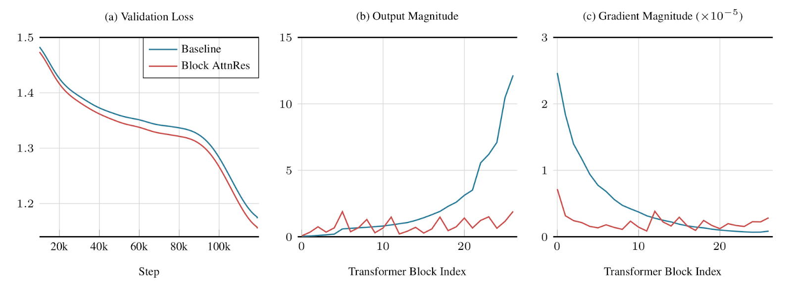
The validation loss of Block AttnRes is consistently lower than the baseline across all steps
The output magnitudes of the layers remain relatively stable, while those of the baseline tend to explode towards the later layers. Hidden state magnitudes grow monotonically with depth, so the deeper layers in baseline are forced to learn large outputs to remain influential. Block AttnRes resolves this with dynamic weighting of incoming residual stream.
The gradient magnitudes also remain stable across layers, indicating that it helps with the vanishing gradient problem. The authors attribute this to the fact that the baseline provides no clear path for gradient flow, while with AttnRes, there is increased competition for probability mass, resulting in a more stable and uniform gradient distribution.
Across standard benchmarks such as MMLU-Pro, GSM8k, etc. Block AttnRes consistently outperforms Baseline
Analyzing AttnRes Patterns
Locality is preserved - most layers tend to only gain access to closest layers before them, but in some cases they do go back further
Layers specialization - The embedding values continue to retain non-trivial weight throughout, especially in pre-attention layers. Pre-MLP inputs show sharper reliance on more recent representations, while pre-attention inputs tend to intermix information from different layers, highlighting that attention layers are routing information across layers while MLPs tend to operate more locally.
Residual Connections as Structured Matrices
All residual variants may be viewed as weighted aggregations over previous layer outputs, referred to as a depth-mixing matrix. The variants of how these residual connections are formed depends on the nature of this matrix, which allows us to interpret them, like we highlighted in our 16th Edition and 14th Edition. Through this, we can also determine what formulation of the kernel function provides the best properties. The reader is invited to refer to section 6 of the paper for a deeper mathematical treatment.
Awesome Machine Learning Summer Schools is a non-profit organisation that keeps you updated on ML Summer Schools and their deadlines. Simple as that.
Have any questions or doubts? Drop us an email! We would be more than happy to talk to you.
Reply